


How statisticians helped the allies win the WWII
Estimating the total number of German tanks produced from a small random sample

How it all started
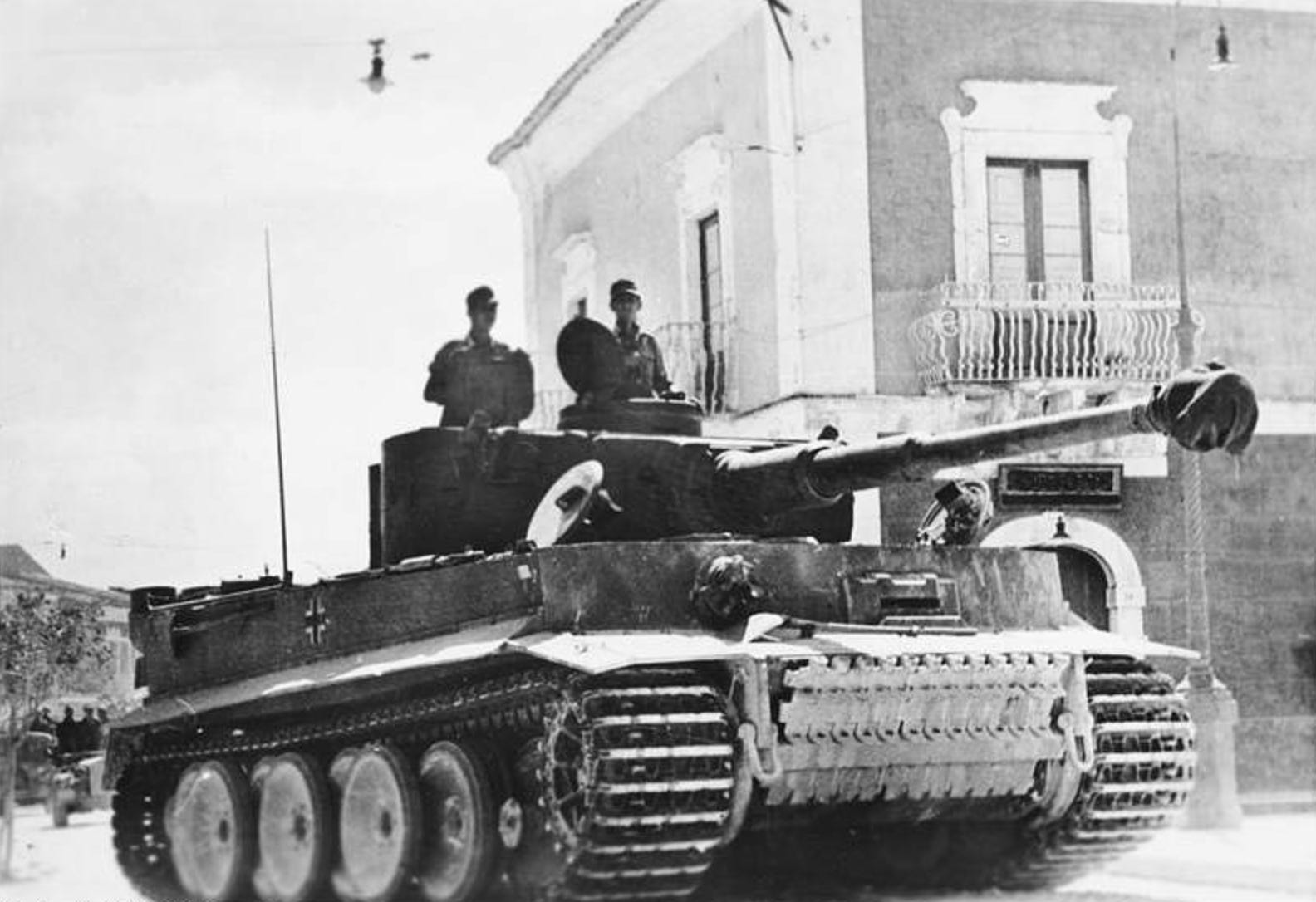
During the WWII, the allies were worried about the capabilities of the new Mark IV and Mark V German Panzer tanks, and how many of those the enemy was capable of producing within a year. Without a reasonable estimate, they were skeptical whether any ground invasion on the war front would be successful. Initially they relied on the ally intelligence a.k.a. “spies” to secretly observe German tank production lines or even manually count tanks on the battlefield, only to realize the estimates were contradictory, hence unreliable.
So they turned to statisticians for help.
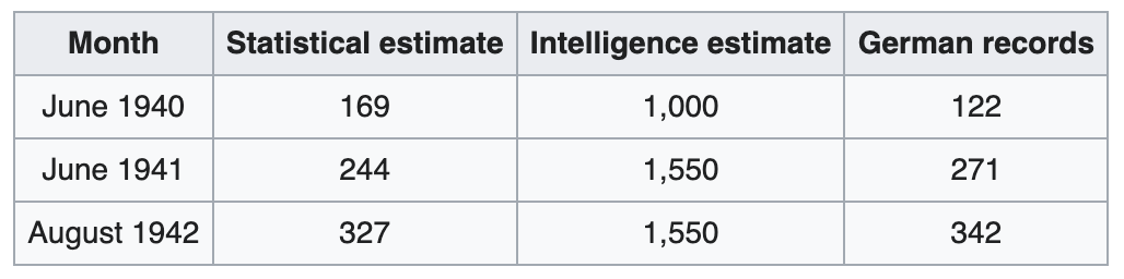
At the time, statisticians had access to one crucial piece of information—the numerical serial numbers on captured Mark V tanks on the battlefield. They believed that Germans being Germans would logically number their tanks in the order they were produced, which turned out to be correct e.g. a tank with the serial number 10 would mean it was the 10th tank in production, and that there wouldn’t be duplicate serial numbers (sampling without replacement). These assumptions along with the assumption that Germans would send tanks randomly to different battlefields (no sampling bias) helped statisticians correctly estimate the true number of German tanks in a given year far better than the ally intelligence (see Figure 1 below).
Let’s see how we can come up with an estimate of the total population size from a limited random sample and compare how the frequentist and the Bayesian approach differ in their estimates1.
Problem setup
Borrowing the German tank example above, say we have the serial numbers of five captured tanks as the following (assume the numbers start from 1) and want to estimate the total number of tanks produced in a given time period using the sample:
Intuitively, we’d look at this and say the total number of tanks is probably a little over 250. I say a little over because the fact we saw four serial numbers below 250 means it's not unlikely we’ll also see numbers higher than 250 had we picked a different sample from the population of all tanks produced. Our goal is to estimate the very overage, the maximum serial number, using a statistical approach.
Formally speaking, assume that the total number of tanks produced in a given time period to be K (this is the unknown we want to estimate), and the five tanks in our sample a.k.a. our “data” to be D.
Frequentist approach
Frequentists assume the unknown parameter of interest, in our case the total number of tanks produced K, is a fixed number (e.g. the total number of tanks produced is either 1000 or not). On average, the total number of tanks produced K, or equivalently, the maximum serial number of all tanks produced is expressed as follows:
Since M = 250 and C = 5, we have K = 250 + 250 / 5 - 1 = 299. We can expect a total of 299 tanks to have been produced. I won’t go through the mathematical derivation of the formula above for the sake of brevity. Intuitively, the very overage (M / C - 1) we add to M is the size of the gap if we had sorted all of the tanks in the sample in a line and imagine if they were evenly spaced a.k.a. the number of unobserved tanks between captured tanks in the sample if they were evenly spaced.

Bayesians to the rescue!
Unlike frequentists, Bayesians would remedy the same problem by putting a distribution around the unknown parameter to quantify their uncertainty (e.g. the total number of tanks produced is a distribution between 250 and 1000, and it’s highly likely to be 300 than others). They combine not only the data D at hand but also so called the priors, which are the assumptions about the unknown parameter K before seeing the data.
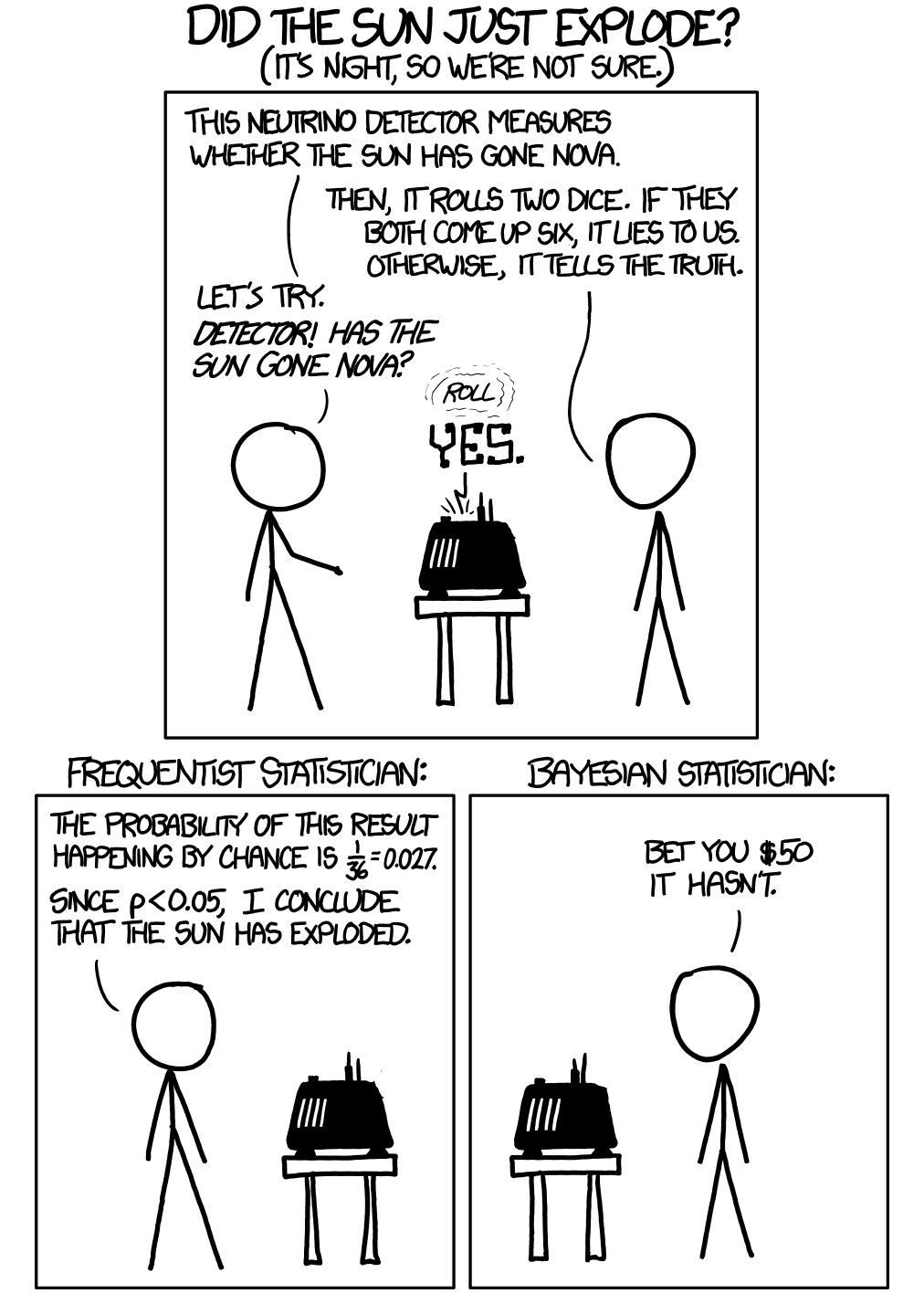
The Bayesian alternative to the frequentist approach tends to be more interpretable and aligns with how humans view the world and update their beliefs over time. Simply said, the prior is the belief you hold before seeing data (e.g. I’ve never seen the sun explode for as long as I’ve been alive, so the prior probability of the sun exploding is nearly zero), and upon seeing data (e.g. sun rising tomorrow again without exploding), you update your prior belief which becomes your posterior (e.g. sun will continue rising the day after tomorrow with a near zero probability of exploding). Updating your belief sequentially one at a time or all at the end ultimately leads you to the same conclusion.
Bayesians want to estimate the (posterior) probability of K given D—that is, P(K|D), how likely do we see different values of K given the data we observe at hand. Using the Bayesian theorem we can decompose P(K|D) as follows:
where P(D|K) refers to the likelihood of observing the five tank sample given the true unknown total number of tanks produced, and P(K) is the prior distribution of the unknown parameter, essentially what we assume to be the likely values of K before observing the data on five tanks. Bayesians would try to come up with the appropriate distributions for both P(D|K) and P(K) to quantify the uncertainty that reflects the real-life situation.
When deciding a reasonable distribution for the likelihood, consider the process in which the data is generated. Given that I know the total number of tanks produced in a given time period is K, the probability of capturing a random German tank on the battlefield should be 1/K, and that 1/K is uniform (constant) for every capture. Statistically speaking, we assume the likelihood to be discrete uniformly distributed with the minimum at 0 and the maximum at the unknown K: Uniform(0, K).

On the other hand, we know that our prior belief over K should be at least as high as the highest tank serial number we observe in the sample (M = 250), but it could also be much higher. Let's also assume P(K) to be discrete uniformly distributed with the minimum at M and the maximum at an arbitrary big number (theoretically speaking, this would be positive infinity but let’s fix it to a large number, say 10000, for the purpose of computing): Uniform(M, ∞).
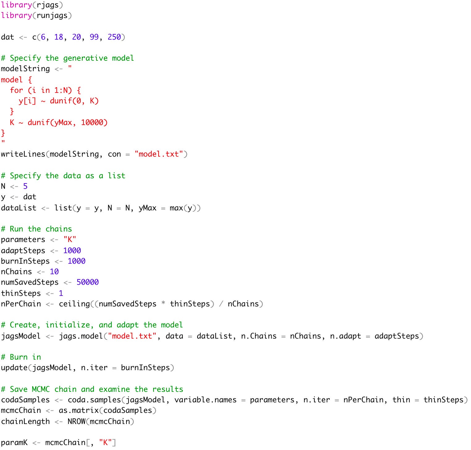
We can derive a closed form solution using combinatorics and the laws of probability, but I’m going to leverage the power of computing in R with JAGS. Essentially you’d randomly sample a value from P(D|K) and a value from P(K) and multiply them to get a value of P(K|D). Repeat this process to get an empirical distribution of P(K|D). JAGS is simply a software that runs this type of complex MCMC (Markov Chain Monte Carlo) simulations from a generative model. You can also use similar softwares like Stan, but JAGS should work fine in most situations.
Check out the full running code I wrote:
By plotting the posterior distribution P(K|D) of the total number of tanks produced, paramK in code, we can see the posterior mode is 264, not 250! The posterior mean is 336, and the median is 297. The 95% highest posterior density interval (HDI) lies between 250 and 536. It’s very unlikely we see numbers in the thousands! The estimate will get better as we capture more tanks. The most probable total number of tanks produced on a given time period is 264. Unsurprisingly this is different from the Frequentist estimate of 299 because in the Bayesian approach we used simulation so the numbers can be a little off, and most importantly, you can use any other distribution to encode your prior belief (e.g. improper uniform prior, negative binomial prior), making the estimate rather subjective.
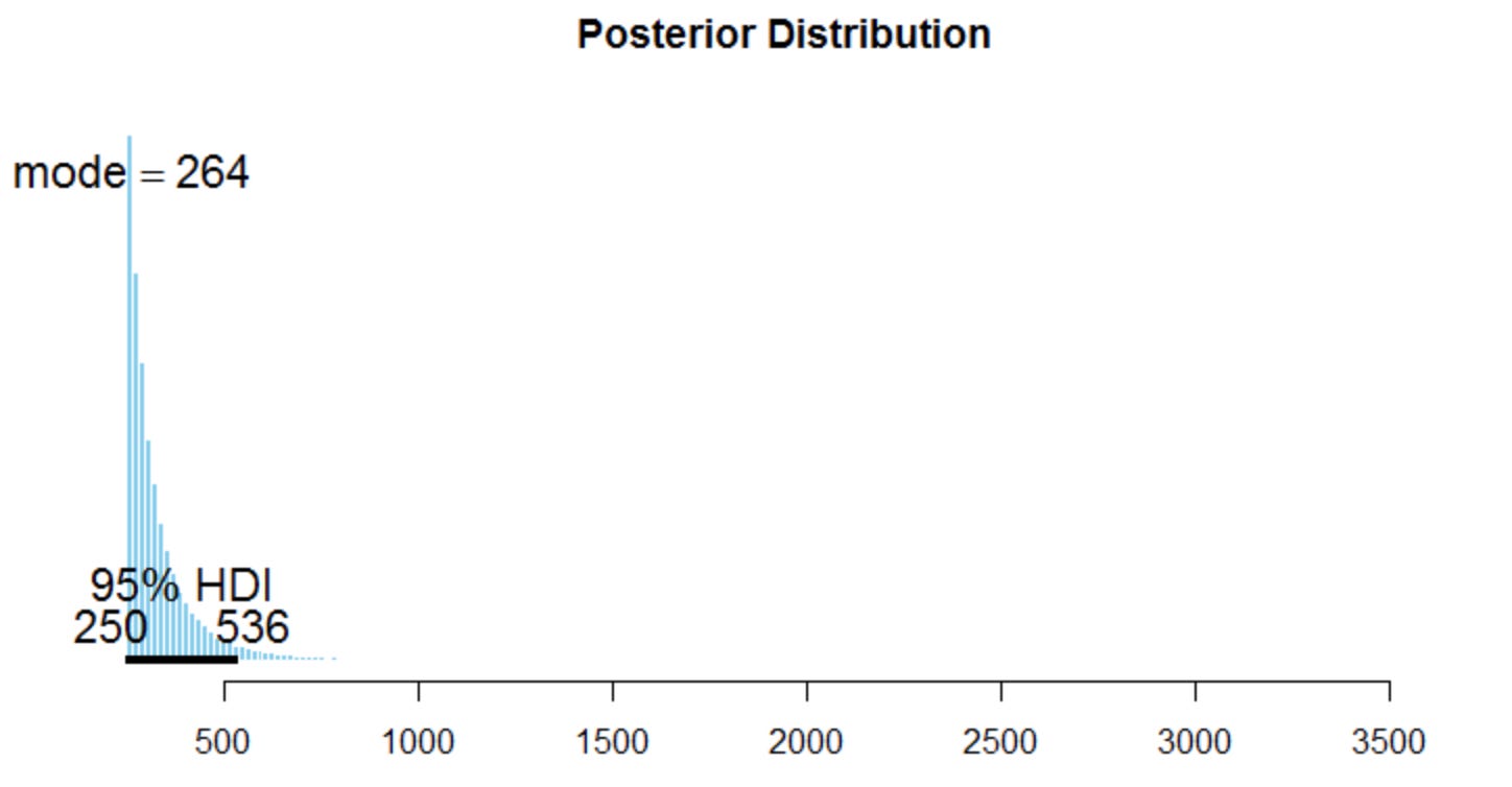
P(K|D). Image by the author.The problem gets more complex if not impossible if Germans decide to revert the serial numbers back to 1 after reaching a certain number, if there is a bias in the sample (e.g. Germans sending certain Mark V tanks to the battlefields in France), or if they use cryptography to mask the serial numbers in some obscure way.
Practical applications
The German tank problem is widely applicable in real-life beyond just war. Examples include but are not limited to:
Estimating the total number of customers at a store in a given day using check IDs in a limited sample of receipts
Estimating the total traffic to a website using a random sample of user IDs
Estimating the total production of parts using a sample of part serial numbers (e.g. iPod, Commodore 64)
Estimating the total number of taxi-cabs in New York city
Parting thoughts
In the world of big data, we often overlook the importance of small data and how we might be giving away more information than we realize even in the small data setting (be careful what you share!). Statisticians have worked for centuries to come up with the incredible methods based on realistic assumptions, and the advent of highly scalable computing softwares has made it possible to support simulating from complex hierarchical models.
Thanks to Rachel Moon on Data Science Doodles for providing helpful feedback on this post and designing the new logo for my publication. The new logo you see on the top left is a “casual” human reading my newsletter. Her contribution is always so much appreciated.
As always, any assumptions and opinions stated here are mine and not representative of my current or any prior employer(s). Note that this post is the unabridged, more polished version of the original post I wrote in my technical blog in 2016.
I assume you have the basic understanding of statistics and the frequentist vs. Bayesian frameworks. If interested in a deeper treatise of the frequentist, likelihoodist, and Bayesian thinking, check out the following resources: